Thursday, October 29, 2015

The Big Squeeze, Or, How We Plan to Get All of Our Legacy Accession Data into ArchivesSpace

Almost two months ago, I wrote a post on what we thought would be thorny issues that would get in the way of importing legacy accession data into ArchivesSpace. This was mostly conjecture, because at that point, we hadn't actively been trying to move data from Beal (a homegrown FileMaker Pro database) to ArchivesSpace. Now that we've had some time to play around with importing legacy accession data, we thought you might like an update on our plan.

The Big Squeeze

Unlike the actual episode from Season 3 of the A-Team, our big squeeze does not involve loan sharks, mob extortion bosses, breaking fingers, sniper assaults (phew!), or Irish pubs (or does it...).
First things first (and this is important), we came up with a name for this project: "The Big Squeeze." Not only is this a nod to an actual episode from Season 3 of the A-Team (the name we've given to the crew here working on ArchivesSpace implementation, that is, the ArchivesSpace Team, or simply, the A-Team), but, as you'll see, it actually fits for some of the way we'll approach importing legacy accession data into ArchivesSpace, namely, squeezing a number of disparate Beal fields into single ArchivesSpace fields.

Big Decision Early On: Don't Worry, Be Happy

Early on, we made the important decision that we simply weren't going to worry about accession records as much as we worried about EADs--we certainly weren't going to spend as much time cleaning them as we did, and still sometimes do, with our EADs. Here's our reasoning: Accession records are relatively static, and serve as mostly internal evidence of a particular transaction or event. EADs, on the other hand, are ever-changing and evolving portals to our collections for humans (internal ones, like archivists, and external ones, like researchers) and systems (and, now, other integrated systems, like DSpace and Hydra!). Likewise, going forward we simply won't be using individual accession records as frequently or even in the same way as we will individual archival descriptions  (there's one exception to this which I'll talk about later). 

As a result, there may be differences, even significant ones, between our legacy conventions and conventions going forward in ArchivesSpace for recording accession information. Our legacy accession records may not be super machine-readable. They won't be connected to associated finding aids. They'll be a little dirty (the horror!). We'll be using some user-defined fields that we won't use going forward. Rather than making significant changes to ArchivesSpace or the accessions importer, we'll just be squeezing a number of Beal fields into one ArchivesSpace field. We'll use Boolean fields rather than create events for some information. We'll use free text fields rather than create actual locations (at least for now). And we're OK with all this. Dare I say we're actually happy with this decision...

The Plan, Stan

The plan. Ignore that stuff on the bottom left.
As you may or may not be able to read in the image above (I don't have the best handwriting), we've formulated a six-step plan:
  1. "Clean" and prep a data dump from Beal.
  2. Map Beal fields to ArchivesSpace fields
  3. Build the JSON that ArchivesSpace expects.
  4. Deal with donors.
  5. Do a dry run.
  6. Do the real thing.
Simple, right?

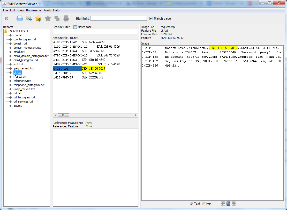
"Clean" and Prep a Data Dump from Beal (Our Homegrown FileMaker Pro Database)

First things first, we need to get our accession data out of our current database. This is a fairly straightforward process, since exporting records from FileMaker Pro is as simple as File --> Export Records, choosing a file name and type, and specifying fields and order for export. I say "fairly" straightforward because of some little quirks about FileMaker Pro we've learned along the way, such as the fact that CSV exports don't include header information, but that there's a mysterious file extension ".mer" that does, that exports contain a bunch of null characters which lead to encoding errors, and that the CSV/MER export by default has a very strange way of recording multiple values in the same field, namely, that it throws the second, third, fourth, etc., values onto the next line(s), all by themselves (and since the CSV reader object in Python is not iterable, it gets tricky to associate orphan values with their proper record).

Then, there's "cleaning" and prepping. Cleaning is in quotes because we aren't actually cleaning all that much. Mostly, "cleaning" is more like straightening, not spring or deep cleaning, preparing the accession records by distilling them down to only the essentials. We made header column names unique (because there were some that weren't), we removed blanks rows, we identified and weeded out meaningless (read, information-less) records, and we filled in missing date information (ArchivesSpace accession records require dates) in most instances by writing a program that automatically guesses a date using context clues and, for about 30 or so, filled them in by hand. In some instances, we also normalized some values for fields with controlled vocabularies--nothing major, though.

Since we're still actively accessioning materials, we're trying to do this in way that will allow us to easily replicate it on future exports from Beal. 

You can read through the code Dallas used to do most of this here; date guessing is here.

Map Beal Fields to ArchivesSpace Fields

Again, this process was fairly straightforward, especially once we made the decision not to worry too much about differences in the ways that Beal and ArchivesSpace model and expect all the components that make up an accession record.
We'll be making fairly extensive use of the user-defined portion of ArchivesSpace accession records. Has anyone changed the labels for these fields? If so, let us know! We're keen to explore this.
We broke this down into a number of categories:
  • Basic Information, like a date and description for an accession, it's size, provenance information, and basic events associated with it, such as whether or not it's receipt has been acknowledged (here's an example of a case where we'll use a Boolean rather than create an event, even though going forward we'll probably use an actual ArchivesSpace event). 
  • Separations, or information about parts of collections we decided not to keep. Here we're talking about fields like description, destruction or return date, location information and volume. When we do have a date associated with a separation, we'll create an actual deaccession record. If we don't, we'll just squeeze all this information into the basic disposition field in ArchivesSpace (again, probably not how we'll use that field going forward, but that's OK!). 
  • Gift Agreement, the status of it, at least. We'll be using a user defined controlled vocabulary field.
  • Copyright, like information on whether it has been transferred. We're going with the tried and true Conditions Governing Use note, although we've been doing a lot of talking lately about how we'll record this type of information going forward, especially for digital collections, and how the rights module in ArchivesSpace, which we'd like to be the system of record for this type of information, isn't really set up to take in full PREMIS rights statements from Archivematica (or RightsStatements.org rights, for that matter) [1]. 
  • Restrictions, which will go to a Conditions Governing Access note (although that same discussion about rights from above applies here as well).
  • Processing, that is, information we record upon accession that helps us plan and manage our processing, information like the difficulty level, the percentage we expect to retain, the priority level, the person who will do it, any notes and the status. Mostly we'll take advantage of the Collection Management fields in ArchivesSpace, and for that last one (the exception I mentioned earlier), we're hopeful that, after an ongoing project to actually determine the status for many backlogged collections, we'll be able to use the events "Processing in Progress" and "Processing Completed". Our thought process here is that this is an instance where we actually will be using accession records actively going forward to determine which accessions still need to be processed; we didn't want different conventions for this pre- and post-ArchivesSpace migration. If that doesn't work out, or it turns out that it will take too much time to straighten out the backlog, we'll be using another user-defined controlled vocabulary field.
  • Unprocessed Location, which will, in the interim, just go to a user-defined free text field. This information has not been recorded consistently, and in the past we haven't been as granular with location information as ArchivesSpace is. We actually like the granularity of location information in ArchivesSpace, though, especially with the affordances of the Yale Container Mangement Plug-in and other recent news. So this is definitely something that will be different going forward, and may actually involve extensive retrospective work.
  • Donors, their names and contact information, as well as some identifiers and numbers we use for various related systems. More on that later. This is also an exception, an instance where we did decide to make a significant change to ArchivesSpace. Check out this post to learn more about the Donor Details Plug-in.
  • Leftovers, or information we won't keep going forward. Hopefully we won't regret this later!
One thing we're considering is trying to make it obvious in ArchivesSpace which records are legacy records and which aren't, perhaps making them read only, so that if conventions change for recording a particular type of information because of the new ArchivesSpace environment, it will be less likely (but not impossible) that archivists will see the old conventions and use those as a model. 

You can check out our final mapping here.

Build the JSON that ArchivesSpace Expects

If you've never played around with it, JSON is awesome. It's nothing fancy, just really well-organized data. It's easy to interact with and it's what you get and post from ArchivesSpace and a number of other applications via their API.
Another famous JSON Jason! [2]
In that mapping spreadsheet you can see how we've mapped Beal fields to the JSON that ArchivesSpace expects. Essentially this involves reading from the CSV and concatenating certain fields (in a way that we could easily parse later if need be), that is, the big squeeze, then making ArchivesSpace deaccession, extent, collection management, user-defined, external documents, date, access restrictions, etc., lists and then JSON. 

You can take a look at that code from Walker here.

Deal with Donors

Donors get their own section. In the end, we hope to do donor agents for accessions the same way we did subject and creator agents (as well as other types of subjects) for EADs, importing them first and linking them up to the appropriate resource/accession later. This won't be too hard, but there are some extenuating circumstances a number of moving parts to this process.

We still have some work to do with some associates of the A-Team here matching up donor information from Beal with donor information from a university system called Dart which is used to track all types of donations to the university, This is a little tricky because we're not always sure which system has the most up-to-date contact information, and because we're not always if Samuel Jackson and Samuel L. Jackson, for example, are the same person (but seriously, we don't have anything from Samuel L. Jackson). The Donor Details plug-in will help us keep this straight (once we're using it!), but in the interim, we have to go through and try to determine which is which. 

We're also currently deciding whether we should actually keep contact information in ArchivesSpace or just point to Dart as the system of record for this information, which is on a much more secure server than ArchivesSpace will be. That presents some problems, obviously, if people need contact information but don't have access to Dart, but we've had internal auditors question our practice of keeping this type of sensitive information in Beal, for example. So that's still an open issue.

Do a Dry Run

It's been done! And it works! It only took an hour and twenty some minutes to write 20,000 accessions (albeit, without donor information)! If you go to the build the JSON link you can also get a peak at how we used the ArchivesSpace API to write all this data to ArchivesSpace. Dallas has also written an excellent post on how to use the ArchivesSpace API more generally which you should also check out.

Do the Real Thing

Sometime between now and April 1, 2016, at the end of our grant, when all the stars align and all the moving parts converge (and once, as a staff we're ready to go forward with accession material and describing it in ArchivesSpace), we'll import or copy legacy accession data into our production environment (this is, by the way, also after we have a production environment...). We're thinking now that we might go live with resources in ArchivesSpace before we go live with accessions, but no firm dates either way as of yet.

Conclusion

Well, that's the plan! What do you think? How did you approach accessions? Are we committing sacrilege by taking a "don't worry, be happy" approach? Let us know via email or on Twitter, or leave a comment below!

[1] Thanks, Ben, for bringing that to our attention.
[2] Stolen from the Internet: http://www.snarksquad.com/wp-content/uploads/2013/01/redranger.gif

Wednesday, October 21, 2015

Methods and Tools for Characterizing and Identifying Records in the Digital Age

Consider this a follow-up to The Work of Appraisal in the Age of Digital Reproduction, one of our most popular blog posts by Mike. According to an extensive review of emerging professional literature, e-discovery search and retrieval in this era of rapid inflation in the amount of electronically stored information is, in short, a challenge. [1] "Traditional" keyword searching, even it's "semantic" variety, has real disadvantages in this environment. Without advanced techniques, keyword searching can be ineffective and often retrieve unrelated records that are not on your topic.

So what's an archivist and/or researcher to do?

According to some, assigning and then browsing by subject headings is the solution to this challenge. [2] Before we all jump on that bandwagon, though (how do you even get to meaningful subject headings in the first place when you have regular born-digital accessions that are many GBs to TBs in size, containing tens of thousands, if not hundreds of thousands, of individual documents), let's walk through a couple of exercises on methods and tools that can be used for characterizing and identifying records in the digital age:
  • Analysis of Drives
  • Digital Forensics
  • Digital Humanities Methods and Tools
    • Text Analysis with Python
    • Named Entity Recognition
    • Topic Modeling

Analysis of Drives

This is a good place to start when you don't know anything at all about what it is you've got. The size of the squares indicates the size of the files and folders in a given drive, while the colors indicate the file type. 

Tool

WinDirStat
WinDirStat is a disk usage statistics viewer and cleanup tool for various versions of Windows.

Exercise

Examining and considering the files in ES-Test-Files or on your computer.

  1. Download and install WinDirStatNote: If you are looking for an alternative for Linux, you are looking for KDirStat and for Mac it would be Disk Inventory X or GrandPerspective.
  2. Open windirstat.exe.
  3. Examine and consider the files in ES-Test-Files (these were assembled for a guest lecture on this topic) or on your computer.
    1. When prompted to Select Drives, select All Local Drives, Individual Drives, or A Folder.
    2. Take a look at the Directory List.
    3. Take a look at the Extension List.
    4. Take a look at the Treemap.
    5. Try coupling the views:
      1. Directory ListTreemap.
      2. TreemapDirectory List.
      3. Directory List | TreemapExtension List.
      4. Extension ListTreemap.
  4. Play around some!

Digital Forensics

Digital forensics encompass the recovery and investigation of material found in digital devices.

Tools

Bulk Extractor Viewer

Bulk Extractor is a program that extracts features such as email addresses, credit card
numbers, URLs, and other types of information from digital evidence media. 

Bulk Extractor Viewer is a user Interface for browsing features that have been extracted via the bulk_extractor feature extraction tool. 

Exercise

Examine the contents of Identity_Finder_Test_Data and identify sensitive data, like social security numbers and credit card numbers. You can also use it to find out what e-mail addresses (correspondence series, anyone?), telephone numbers and website people visit (or at least show up in text somewhere), and how often.

  1. Download and install Bulk Extractor. Note: Windows users should use the development build located here.
  2. Open BEViewerLauncher.exe.
  3. Under the Tools menu, select Run bulk_extractor…, or hit Ctrl + R.
  4. When prompted to Run bulk_extractor, scan a Directory of Files and navigate to Identity_Finder_Test_Data.
  5. Create an Output Feature Directory such as Identify_Finder_Test_Data_BE_Output.
  6. Take a look at the General Options.
  7. Take a look at the Scanners. Note: More information on bulk_extractor scanners is located here.
  8. Submit Run.
  9. When it’s finished, open the Output Feature Directory and verify that files have been created. Some will be empty and others will be populated with data.
  10. In Bulk Extractor Viewer select the appropriate report from Reports.
  11. Take a look at the Feature Filter.
  12. Take a look at the Image.
  13. Play around some!
And there's more! This tool is used in BitCurator and we're incorporating this tool and related functionality into the Appraisal and Arrangement tab:
File:ATab-PII.png
SSNs identified!

Digital Humanities Methods and Tools

These, arguably, are emerging tools for characterizing and identifying records. Still, whether they are used in conjunction with researchers to answer new and exciting research questions or to create new interfaces to collections, or to decrease the amount of time between accession and access (with the obligatory note that they don't replace trained, human effort to do the work of description) for gigantic collections of born-digital material that you know next to nothing about, these methods and tools are worth a look.

Text Analysis with Python

Method

Text Analysis is automated and computer-assisted method of extracting, organizing, and consuming knowledge from unstructured text.

Tools

Python is a widely used general-purpose, high-level programming language.

The Natural Language Toolkit (NLTK) is a leading platform for building Python programs to work with human language data.

Exercise

  1. Download and install Python. Note: Mac users, Python will be pre-installed on your machines. You may also choose to install Python's NumPy and Matplotlib packages (and all their dependencies). This isn't strictly necessary, but you’ll need them in order to produce the graphical plots we'll be using.
  2. Download and install NLTK.
  3. Open Interactive DeveLopment Environment (IDLE), or any command line or terminal.
Getting started with NLTK:
    1. Type: import nltk
    2. Type: nltk.download()
    3. At the NLTK Downloader prompt, select all (or book, if you are concerned about size) and Download.
    4. Exit the NLTK Downloader.
    5. Type: from nltk.book import *
    6. Type: text1, text2, etc. to find out about these texts.
Searching text:
    1. Type: text1.collocations()to return frequent word combinations.
    2. Type: text1.concordance(“monstrous”)
    3. Play around some! For example, look for nation, terror, and god in text4 (Inaugural Address Corpus) and im, ur, and lol in text5 (NPS Chat Corpus).
    4. Type: text1.similar(“monstrous”)
    5. Type: text2.similar(“monstrous”)
    6. Observe that we get different results for different texts. Austen uses this word quite differently from Melville; for her, monstrous has positive connotations, and sometimes functions as an intensifier like the word very.
    7. Type: text2.common_contexts([“monstrous”, “very”])
    8. Play around some! Pick another pair of words and compare their usage in two different texts, using the similar() and common_contexts() functions.
    9. Type: text4.dispersion_plot([“citizens”, “democracy”, “freedom”, “duties”, “America”])

    ../images/inaugural.png
    Lexical Dispersion Plot for Words in U.S. Presidential Inaugural Addresses: This can be used to investigate changes in language use over time.
Counting vocabulary:
  1. Type: len(text3) to get the total number of words in the text.
  2. Type: set(text3) to get all unique words in a text.
  3. Type: len(set(text3)) to get the total number of unique words in the text, including differences in capitalization.
  4. Type: text3_lower = [word.lower() for word in text3] to make all words lowercase. Note: This is so that capitalized and lowercase versions of the same word don't get counted as two words.
  5. Type: from nltk.corpus import stopwords
  6. Type: stopwords = stopwords.words(“english”)
  7. Type: text3_clean = [word for word in text3_lower if word not in stopwords] to remove common words from text.
  8. Type: len(text3_clean) / len(set(text3_clean)) to get total words divided by set of unique words, or lexical diversity.
And there’s more! Here's a couple of examples of lexical diversity in action:
This plot shows lexical diversity over time for the Michigan Technic, a collection we've digitized here at the Bentley, using Seaborn, a Python visualization library based on matplotlib. Not much of a trend either way, although I'm not sure what happened in 1980.

Not exactly an archival example, but one of my favorites nonetheless. The Largest Vocabulary in Hip Hop: Rappers, Ranked by the Number of Unique Words in their Lyrics. The Wu Tang Association is not to be trifled with.
Frequency distributions:
  1. Type: fdist1 = nltk.FreqDist(text1)
  2. Type: print fdist1
  3. Type: fdist1.most_common(50)
  4. Type: fdist1.[“whale”]
  5. Type: fdist1.plot(50, cumulative=True)
  6. Play around some! Try the preceding frequency distribution example for yourself.
  7. Type: fdist1.hapaxes() to view the words in the text that occur only once.
../images/fdist-moby.png
Cumulative Frequency Plot for 50 Most Frequently Words in Moby Dick: these account for nearly half of the tokens.
And there's more! Here's an example of a frequency distribution in action:
A word cloud (an alternative way to visualize frequency distributions), again for the Michigan Technic. If you couldn't tell from "engineer" and "engineers" and "engineering" (not to mention "men" and "man" and "mr."), this is an engineering publication.

Named Entity Recognition [3]

Method

Named Entity Recognition (NER) seeks to locate and classify elements in text into predefined categories such as the names of persons, organizations, locations, expressions of times, quantities, monetary values, percentages, etc.

Tool

Stanford Named Entity Recognizer
Stanford Named Entity Recognizer (Stanford NER) is a Java implementation of Named Entity Recognizer. Named Entity Recognition (NER) is method that allows automatic labeling of things like people, organizations, and geographic locations in unstructured text.

Exercise

  1. Download and unzip Stanford NER.
  2. Download and unzip looted_heritage_reports_txt.zip.
  3. Open stanford-ner.jar.
  4. Under Classifier click Load CRF From File.
  5. Navigate to Stanford-ner-2015-04-20/classifiers/english.all.3class.distsim.crf.ser.gz.
  6. Under the File menu, click Open File.
  7. Navigate to any file in the unzipped looted_heritage_reports_txt folder (or use any text file).
  8. Click Run NER.
  9. Observe that every entity that Stanford NER is able identify is now tagged. 
  10. Under the File menu, click Save Tagged File As …
And there's more! No one's arguing that this is perfect, but I think it does a fairly good first pass at identifying the people, places and organizations mentioned in a piece of text. It wouldn't take much to take those tagged files, create lists of unique people, places, and organizations, and do stuff like this:
ePADD, a software package developed by Stanford University's Special Collections & University Archives, supports archival processes around the appraisal, ingest, processing, discovery, and delivery of email archives. This image previews it's natural language processing functionality.
    Those lists of places could be geo-coded and turned into something like this, a map of Children's Traffic Fatalities in Detroit 2004-2014 (notice how the size of the dot indicates frequency).

Topic Modeling

Topic modeling is a procedure used to derive topical content from documents. One of the 
most frequently used tools for topic modeling is MALLET, which provides this 
definition:  
Topic models provide a simple way to analyze large volumes of unlabeled text. A "topic" consists of a cluster of words that frequently occur together. Using contextual clues, topic models can connect words with similar meanings and distinguish between uses of words with multiple meanings.

Tool

Topic Modeling Tool
Whereas MALLET is a command-line tool, Topic Modeling Tool provides an interactive interface

Exercise

  1. Download Topic Modeling Tool.
  2. Open TopicModelingTool.jar.
  3. Click Select Input File or Dir and navigate to the unzipped looted_heritage_reports_txt folder (or use any folder of text files).
  4. Create a new folder on your computer to hold the topic model data you will create, such as looted_heritage_reports_text_output.
  5. Click Select Output Dir and select the new folder.
  6. For Number of topics: enter 15.
  7. Click Learn Topics.
  8. Take a look at the output_csv directory.
  9. Take a look at the output_html directory.
  10. Explore the Advanced… options.
This actual collection of looted heritage reports was used in Mining the Open Web with 'Looted Heritage'. If you scroll down to Findings - Topic Modeling, you can see how this author created descriptive labels for the key words discovered using MALLET (like you just did!) in a draft of a publication. A similar process could be used to turn topics into subject headings.

And there's more! Take a look at this example of topic modeling in action:
Topic Model Stacked Bar Graphs from Quantifying Kissinger.

Conclusion

What do you think? Could analysis of drives, digital forensics or digital humanities methods and tools be incorporated into your workflow, or have they been? How else are you overcoming the keyword searching problem? Is the keyword searching problem even a problem at all? What do your researchers think? Let us know!


[1] At least according to this article, and this one as well. Yes, I was very thorough...
[2] Maybe. Possibly. Not as much as we like to think, probably. According to our most recent server logs for September (with staff users and bots filtered out), only 0.25% of users of our finding aids looked at our subject headings. That says something, even if it is true that our current implementation of subject headings is rather static.
[3] The following two sections contain content developed by Thomas Padilla and Devin Higgins for a Mid-Michigan Digital Practitioners workshop, Leveraging Digital Humanities Methods and Tools in the Archive. Thanks, guys!

Monday, October 5, 2015

Tools for the programming archivist: ead manipulation with python and lxml

LXML is an awesome python tool for reading and editing xml files, and we've been using it extensively during the grant period to do programmatic cleanup to our legacy EAD files. To give an example of just how powerful the library is, late last week we ran a script to make tens of thousands of edits to all of our ~2800 EAD files, and it took all of 2 minutes to complete. This would have been an impossible task to complete manually, but lxml made it easy.

We want to share the love, so in this post we'll be walking through how we use the tool to make basic xml edits, with some exploration of the pitfalls and caveats we've encountered along the way.

Setup

Assuming you already have a version of python on your system, you'll first need to install the lxml library

In an ideal world, that should be as easy as running "pip install lxml" from a command-line. If that doesn't work, you have a few options based on what your OS is:

  1. If you're on a mac, try "sudo pip install lxml", and type in your password when prompted.
  2. If you're on windows, you may need to run a special installer. Try this official version. You may be required to first install these two dependencies: libxml2 and libxslt.

We'll also need an ead file (or directory of files) to work on. For this demo we'll be using the ead for the UMich gargoyle collection (raw data here).

Basic usage


Parsing the ead file

First, we need to point lxml to the input ead.

Now we have an lxml "etree" or "element tree" object to work with, and we can do all sorts of things with it. From this parent tree, we can now select individual tags or groups of tags in the ead document to perform actions on, based on just about any criteria we can come up with. To do this we'll first need to use an "xpath" search:


Using xpaths

There are a few things to know about lxml's xpath function:

First, it takes input in the xpath language standard, which is a standardized way to designate exact locations within an xml file. For example, the above search returns a list of every extent tag appearing in the ead file -- the double slashes at the beginning mean that it should look for those tags anywhere in the document. If I wanted to be more specific, I could use an exact search, which would be something like "/ead/archdesc/did/physdesc/extent". We will only be going into basic xpath usage here, but the language is ridiculously powerful - if you're curious as to more advanced things you can do with it, check out this tutorial.

Second, an xpath search always returns a list, even if only one result is found. It's really easy to forget this while writing a quick script, so if you're getting errors talking about your code finding a list when it didn't expect one, that's probably the reason.

A few more xpath examples:


Accessing individual tags and their data

The xpath search will give us a list of results, but to look at or edit any individual tag we'll need to grab it out of the search results. Once we have an individual element (lxml's representation of the tag) we can start to access some of its data:


Tag manipulation

Ok! Now that we know how to get at subsections of the ead file, we can start doing some programmatic edits. In our experience, our edits fall into one of just a few categories of possible changes:

  • editing tag text
  • editing tag types
  • moving tags around
  • creating new tags
  • deleting old tags
  • editing attributes

We'll go through each of these and give some examples and practical tips from our own experience working with EADs at the Bentley.


Editing tag text

This is usually a fairly straightforward task, though there is one big exception when dealing with groups of inline tags. A simple straightforward example:

This gets more complicated when you're dealing with a tag like the following:

<unittitle>Ann Arbor Township records, <unitdate>1991-2002</unitdate>, inclusive</unittitle>

Trying to access unittitle.text here will only return "Ann Arbor Township records, " and ignore everything afterwards. There is no easy way around this through lxml itself, so in these cases we've found it easiest to just convert the whole element to a string using the etree.tostring() method, doing some normal python string manipulation on that result, then converting it back into an element using etree.fromstring() and inserting it back into the ead file. That looks a little like this:

Don't worry if some of that didn't make sense -- we'll be going over more of the creating, inserting, and moving elements later on.


Editing tag types

The most straight-forward of edits. Here's an example:


Editing tag attributes

Attributes are accessed by calling .attrib on the element, which returns a python dictionary containing a set of keys (the attribute names) and their respective values:

Editing the attributes is a pretty straightforward task, largely using python's various dictionary access methods:


Deleting tags

Here you will need to access the parent tag of the tag to be deleted using the element's .getparent() method:


Creating tags

There are two primary ways of going about this - one long and verbose, and the other a kind of short-hand built in to lxml. We'll do the long way first:

The alternate method is to use lxml's element builder tool. This is what that would look like:


Moving tags around

The easiest way to do this is to treat the element objects as if they were a python list. Just like python's normal list methods, etree elements can use .insert, .append, .index, or .remove. The only gotcha to keep in mind is that lxml never copies elements when they are moved -- the singular element itself is removed from where it was and placed somewhere else. Here's a move in action:


Saving the results

Once you've made all the edits you want, you'll need to write the new ead data to a file. The easiest way we've found to do this is using the etree.tostring() method, but there are a few important caveats to note. .tostring() takes a few optional arguments you will want to be sure to include: to keep your original xml declaration you'll need to set xml_declaration=True, and to keep a text encoding statement, you'll need encoding="utf-8" (or whatever encoding you're working with):

We can also pretty-print the results, which will help ensure the ead file has well-formed indentation, and is generally not an incomprehensible mess of tags. Because of some oddities in the way lxml handles tag spacing, to get pretty-print to work you'll need to add one extra step to the the input file parsing process:

Note that the new parser will effectively remove all whitespace (spaces and newlines) between tags, which can cause problems if you have any complicated tag structure. We had some major issues with this early on, and ended up writing our own custom pretty-printing code on top of what is already in lxml, which ensures that inline tags keep proper spacing (as in, <date>1926,</date> <date>1965</date> doesn't become <date>1926,</date><date>1965</date>), and to prevent other special cases like xml lists from collapsing into big blocks of tags. Anyone is welcome to use or adapt what we've written - check it out here!


Thanks for reading along! We've found lxml to be indispensable in our cleanup work here at the Bentley, and we hope you'll find it useful as well. And if you have any thoughts or use any other tools in your own workflows we'd love to hear about them -- let us know in the comments below!